4/08/2011

04-08-11 - Friday Filters

So in the last post we made the analysis filters for given synthesis filters that minimize L2 error.

Another common case is if you have a set of discrete data and wish to preserve the original values exactly. That is, you want to make your synthesis interpolate the original points.

(obviously some synthesis filters like sinc and box are inherently interpolating, but others like gauss and cubic are not).

So, the construction proceeds as before, but is actually simpler. Rather than using the hat overlaps we only need the values of the synthesis at the lattice points. That is :


Given synthesis/reconstruction filter S(t)
and discrete points P_i
Find points Q_i such that :

f(t) = Sum_i Q_i * S(t - i)

f(j) = P_j for all integers j

We can write this as a matrix equation :

Sij = S(j - i) = S(i - j)

S * Q = P

note that S is band-diagonal. This is the exact same kind of matrix problem that you get when solving for B-splines.

In general, if you care about the domain boundary effects, you have to construct this matrix and solve it somehow. (matrix inversion is a pretty bad way, there are fast ways to solve sparse band-diagonal matrices).

However, if the domain is large and you don't care too much about the boundary, there's a much simpler way. You just find S^-1 and look at a middle row. As the domain size goes to infinity, all the rows of S^-1 become the same. For finite domain, the first and last rows are weird and different, but the middle rows are about the same.

This middle row of S^-1 is the analysis filter.


A = middle row of S^-1

Q = A <conv> P

Q_i = Sum_j A(i-j) P_j

note A is only defined discretely, not continuously. Now our final output is :

f(t) = Sum_i Q_i * S(t - i)

f(t) = Sum_i Sum_j A(i-j) P_j * S(t - i)

f(t) = Sum_j C(t-j) * P_j

C(t) = Sum_i A(i) * S(t-i)

where C is the combined analysis + synthesis filter. The final output is just a simple filter applied to the original points.

For example, for the "canonical cubic" synthesis , (box convolved thrice), we get :


cubic analysis :
const float c_filter[11] = { -0.00175, 0.00876, -0.03327, 0.12434, -0.46410, 1.73205, -0.46410, 0.12434, -0.03327, 0.00876, -0.00175 };
chart : 

(A is 11 wide because I used an 11x11 matrix; in general it's infinitely wide, but gets smaller as you go out)

The synthesis cubic is piece-wise cubic and defined over four unit intervals from [-2,2]
The combined filter is piece-wise cubic; each unit interval is a linear combo of the 4 parts of synthesis

{ ADDENDUM : BTW this *is* the B-spline cubic; see for example : Neil Dodgson Image resampling page 128-129 ; the coefficients are exactly the same }

So, you could do all this work, or you could just use a filter that looks like "combined" from the start.


gaussian analysis :
const float c_filter[11] = { -0.00001, 0.00008, -0.00084, 0.00950, -0.10679, 1.19614, -0.10679, 0.00950, -0.00084, 0.00008, -0.00001 };
chart : 

mitchell1 analysis :
const float c_filter[11] = { -0.00000, 0.00002, -0.00028, 0.00446, -0.07115, 1.13389, -0.07115, 0.00446, -0.00028, 0.00002, -0.00000 };
chart : 

Now, not surprisingly all of the "combined" filters look very similar, and they all look rather a lot like windowed sincs, because there simply aren't that many ways to make interpolating filters. They have to be = 1.0 at 0, and = 0.0 at all other integer locations.

ADDENDUM : well, I finally read the Nehab/Hoppe paper "Generalized Sampling" , and guess what, it's this. It comes from a 1999 paper by Blu et.al. called "Generalized Interpolation: Higher Quality at no Additional Cost".

The reason they claim it's faster than traditional filtering is that what we have done is to construct a sinc-like interpolating filter with wide support, which I call "combined", which can be separated into a simple compact "synthesis" filter, and a discrete matrix (S^-1). So for the case where you have only a few sets of data and you sample it many times (eg. texture in games), you can obviously implement this quickly by pre-applying the discrete matrix to the data, so you no longer have samples of the signal as your pixels, instead you have amplitudes of synthesis basis functions (that is, you store Q in your texture, not P). Now you can effectively sample the "combined" filter by applying only the "synthesis" filter. So for example Nehab/Hoppe suggests that you can do this fast on the GPU by using a GPU implementation of the cubic basis reconstruction.

Both of the papers are somewhat misleading in their claims of "higher quality than traditional filtering". You can of course compute a traditional linear filter that gives the same result, since their techniques are still just linear. They are higher quality *for the same complexity of filter* , and only if you have pre-done the S^-1 multiplication. The speed advantage is in being able to precompute the S^-1 multiplication.

4/07/2011

04-07-11 - Help me I can't stop

Some common synthesis filters and their corresponding analysis filter :
BEGIN review

if you want to approximate f(t) by

Sum_i P_i * synthesis(t-i)

you can find the P's by :

P_i = Convolve{ f(t) analysis(t-i) }

END review
a note on the method :

BEGIN note

the H overlap matrix was computed on a 9x9 domain
because my matrix inverse is ungodly slow

for sanity checking I compared to 11x11 a few times and found the difference to be small
for example :

linear filter invH 9x9 :

0.0038,-0.0189,0.0717,-0.2679,1.0000,-0.2679,0.0717,-0.0189,0.0038

linear filter invH 11x11 :

-0.0010,0.0051,-0.0192,0.0718,-0.2679,1.0000,-0.2679,0.0718,-0.0192,0.0051,-0.0010

(ideally I would use a very large matrix and then look at the middle row, because that is
where the boundary has the least effect)

for real use in a high precision environment you would have to take the domain boundary more seriously

also, I did something stupid and printed out the invH rows with the maximum value scaled to 1.0 ; the
unscaled values for linear are :

-0.0018,0.0088,-0.0333,0.1243,-0.4641,1.7320,-0.4641,0.1243,-0.0333,0.0088,-0.0018

but, I'm not gonna redo the output to fix that, so the numbers below have 1.0 in the middle.

END note

For box synthesis, analysis is box.

linear : invH middle row : = 
0.0038,-0.0189,0.0717,-0.2679,1.0000,-0.2679,0.0717,-0.0189,0.0038,
-0.0010,0.0051,-0.0192,0.0718,-0.2679,1.0000,-0.2679,0.0718,-0.0192,0.0051,-0.0010,

(note: we've see this linear analysis filter before when we talked about how to find the optimum image such that when it's bilinear interpolated you match some original as well as possible)

quadratic invH middle row : = 
0.0213,-0.0800,0.1989,-0.4640,1.0000,-0.4640,0.1989,-0.0800,0.0213,

gauss-unity : invH middle row : = 
0.0134,-0.0545,0.1547,-0.4162,1.0000,-0.4162,0.1547,-0.0545,0.0134,

note : "unity" means no window, but actually it's a rectangular window with width 5 ; the gaussian has sdev of 0.5

sinc half-width of 20 :

sinc-unity : invH middle row : = 
0.0129,-0.0123,0.0118,-0.0115,1.0000,-0.0115,0.0118,-0.0123,0.0129,

note : obviously sinc is its own analysis ; however, this falls apart very quickly when you window the sinc at all, or even just cut it off when the values get tiny :

sinc half-width of 8 :

sinc-unity : invH middle row : = 
0.0935,-0.0467,0.0380,-0.0354,1.0000,-0.0354,0.0380,-0.0467,0.0935,

lanczos6 : invH middle row : = 
0.0122,-0.0481,0.1016,-0.1408,1.0000,-0.1408,0.1016,-0.0481,0.0122,

lanczos4 : invH middle row : = 
0.0050,-0.0215,0.0738,-0.1735,1.0000,-0.1735,0.0738,-0.0215,0.0050,

Oh, also, note to self :

If you print URLs to the VC debug window they are clickable with ctrl-shift, and it actually uses a nice simple internal web viewer, it doesn't launch IE or any such shite. Nice way to view my charts during testing.

ADDENDUM : Deja vu. Rather than doing big matrix inversions, you can get these same results using Fourier transforms and Fourier convolution theorem.

cbloom rants 06-16-09 - Inverse Box Sampling
cbloom rants 06-17-09 - Inverse Box Sampling - Part 1.5
cbloom rants 06-17-09 - Inverse Box Sampling - Part 2

4/06/2011

04-06-11 - And yet more on filters

In the comments of the last post we talked a bit about reconstruction/resampling. I was a bit confounded, so I worked it out.

So, the situation is this. You have some discrete pixels, P_i. For reconstruction, each pixel value is multiplied by some continuous impulse function which I call a "hat", centered at the pixel center. (maybe this is the monitor's display response and the output value is light, or whatever). So the actual thing you care about is the continuous output :


Image(t) = Sum_i P_i * hat( t - i)

I'll be working in 1d here for simplicity but obviously for images it would be 2d. "hat" is something like a box, linear, cubic, gaussian, whatever you like, presumably symmetric, hopefully compact.

Okay, so you wish to resample to a new set of discrete values Q_i , which may be on a different lattice spacing, and may also be reconstructed with a different basis function. So :


Image'(t) = Sum_j Q_j * hat'( t - r*j )

(where ' reads "prime). In both cases the sum is on integers in the image domain, and r is the ratio of lattice spacings.

So what you actually want to minimize is :


E = Integral_dt {  ( Image(t) - Image'(t) )^2 }

Well to find the Q_j you just do derivative in Q_j , set it to zero, rearrange a bit, and what you get is :


Sum_k H'_jk * Q_k = Sum_i R_ij * P_i

H'_jk = Integral_dt { hat'(t-r*j) * hat'(t-r*k) }

R_ij = Integral_dt { hat'(t-r*j)) * hat(t-i) }

or obviously in matrix notation :

H' * Q = R * P

"H" (or H') is the hat self-overlap matrix. It is band-diagonal if the hats are compact. It's symmetric, and actually

H_ij = H( |i-j| )

that is, it only depends on the absolute value of the difference :

H_ij = 
H_0 H_1 H_2 ...
H_1 H_0 H_1 H_2 ...
H_2 H_1 H_0 ...

and again in words, H_i is the amount that the hat overlaps with itself when offset by i lattice steps. (you could normalize the hats so that H_0 is always 1.0 ; I tend to normalize so that h(0) = 1, but it doesn't matter).

If "hat" is a box impulse, then H is the identity matrix (H_0 = 1, else = 0). If hat is the linear tent, then H_0 = 2/3 and H_1 = 1/6 , if hat is Mitchell1 (compromise) the terms are :


H_0 : 0.681481
H_1 : 0.176080
H_2 : -0.017284
H_3 : 0.000463

While the H matrix is very simple, there doesn't seem to be a simple closed form inverse for this type of matrix. (is there?)

The R matrix is the "resampling matrix". It's the overlap of two different hat functions, on different spacings. We can sanity check the trivial case, if r = 1 and hat' = hat, then H = R, so Q = P is the solution, as it should be. R is also sparse and sort of "band diagonal" but not along the actual matrix diagonal, the rows are shifted by steps of the resize ratio r.

Let's try a simple case. If the ratio = 2 (doubling), and hat and hat' are both linear tents, then :


H_0 = 2/3 and H_1 = 1/6 , and the R matrix has sparse rows made of :

...0..., 0.041667, 0.250000, 0.416667, 0.250000, 0.041667 , .... 0 ....

Compute  H^-1 * R =

makes a matrix with rows like :

0 .. ,0.2500,0.5000,0.2500,0 ..

which is a really complicated way to get our triangle hat back, evaluated at half steps.

But it's not always that trivial. For example :


if the hat and hat' are both cubic, r = 2, 

H (self overlap) is :

0 : 0.479365
1 : 0.236310
2 : 0.023810
3 : 0.000198

R (resize overlap) is :

0 : 0.300893
1 : 0.229191
2 : 0.098016
3 : 0.020796
4 : 0.001538
5 : 0.000012

and H^-1 * R has rows of :

..0..,0.0625,0.2500,0.3750,0.2500,0.0625,..0..

which are actually the values of the standard *quadratic* filter evaluated at half steps.

So the thing we get in the end is very much like a normal resampling filter, it's just a *different* one than if you just evaluated the filter shape. (eg. the H^-1 * R for a Gaussian reconstruction hat is not a Gaussian).

As noted in the previous comments - if your goal is just to resize an image, then you should just choose the resize filter that looks good to your eyes. The only place where this stuff might be interesting is if you are trying to do something mathematical with the actual image reconstruction. Like maybe you're trying to resample from monitor pixels to rod/cone pixels, and you have some a-priori scientific information about what shape reconstruction functions each surface has, so your evaluation metric is not ad-hoc.

.. anyhoo, I'm sure this topic has been covered in academic papers so I'm going to leave it alone.

ADDENDUM : another example while I have my test app working.


Gaussian filter with sdev = 1/2, evaluated at half steps :

1.0000,0.6065,0.1353,0.0111,0.0003,...

The rows of (H^-1 * R) provide the resizing filter :

1.0000,0.5329,0.0655,0.0044,-0.0007,...

which comes from :

filter self overlap (H) :
0 : 0.886227
1 : 0.326025
2 : 0.016231
3 : 0.000109
4 : 0.000000
5 : 0.000000

filter resample overlap (R) :
0 : 1.120998
1 : 0.751427
2 : 0.226325
3 : 0.030630
4 : 0.001862


Let me restart from the beginning on the more general case :

Say you are given a continuous function f(t). You wish to find the discrete set of coefficients P_i such that under simple reconstruction by the hats h(t-i) , the L2 error is minimized (we are not doing simple sampling such that P_i = f(i)). That is :


the reconstruction F is :

F(t) = Sum_i P_i * h(t-i)

the error is :

E = Integral_dt { ( f(t) - F(t) ) ^2 }

do derivative in P_i and set to zero, you get :

Sum_j H_ij * P_j = Integral_dt { f(t) * h(t-i) }

where H is the same hat self-overlap matrix as before :

H_ij = h_i <conv> h_j

(with h_i(t) = h(t-i) and conv means convolution obviously)

or in terse notation :

H * P = f <conv> h

(H is a matrix, P is a vector )

rearranging you can also say :

P_j = f <conv> g

if

g_i(t) = Sum_j [ H^-1_ij * h(t-j) ]

what we have found is the complementary basis function for h. h (the hat) is like a "synthesis wavelet" and g is like an "analysis wavelet". That is, once you have the basis set g, simple convolution with the g's produces the coefficients which are optimal for reconstruction with h.

Note that typically H^-1 is not compact, which means g is not compact - it has significant nonzero value over the entire image.

Also note that if there is no edge to your data (it's on infinite domain), then the g's are just translations of each other, that is, g_i(t) = g_0(t-i) ; however on data with finite extent this is not the case (though the difference is compact and occurs only at the edges of the domain).

It should be intuitively obvious what's going on here. If you want to find pixel P_i , you take your continuous signal and fit the hat at location i and subtract that out. But your neighbors' hats also may have overlapped in to your domain, so you need to compensate for the amount of the signal that they are taking, and your hat overlaps into your neighbors, so choosing the value of P_i isn't just about minimizing the error for that one choice, but also for your neighbors. Hence it becomes non-local, and very much like a deconvolution problem.

4/04/2011

04-04-11 - Yet more notes on filters

Topics for today :

N-way filters

symmetry of down & up

qualitative notes

comb sampling

1. N-way filters. So for a long time cblib has had good doublers and halvers, but for non-binary ratios I didn't have a good solution and I wasn't really sure what the solution should be. What I've been doing for a long time has been to use doublers/halvers to get the size close, then bilinear to get the rest of the way, but that is not right.

In fact the solution is quite trivial. You just have to go back to the original concept of the filters as continuous functions. This is how arbitrary float samplers work (see the Mitchell papers for example).

Rather than a discrete filter, you use the continuous filter impulse. You put a continuous filter shape at each pixel center, multiplied by the pixel value. Now you have a continuous function for your whole image by just summing all of these :


Image(u,v) = Sum[ all pixels ] Pixel[i,j] * Filter_func( u - i, v - j )

So to do an arbitrary ratio resize you just construct this continuous function Image, and then you sample it at all the fractional u,vs.

Now, because of the "filter inversion" principle that I wrote about before, rather than doing this by adding up impulse shapes, you can get the exact same output by constructing an impulse shape and convolving it with the source pixels once per output pixel. The impulse shape you make should be centered on the output pixel's position, which is fractional in general. This means you can't precompute any discrete filter taps.

So - this is cool, it all works. But it's pretty slow because you're evaluating the filter function many times, not just using discrete taps.

There is one special case where you can accelerate this : integer ratio magnifications or minifications. Powers of two obviously, but also 3x,5x, etc. can all be fast.

To do a 3x minification, you simply precompute a discrete filter that has a "center width" of 3 taps, and you apply it in steps of 3 to make each output pixel.

To do a 3x magnification, you need to precompute 3 discrete filters. The 3 filters will be applied at each source pixel location to produce 3 output pixels per source pixel. They correspond to the impulse shape offset by the correct subpixel amounts (for 3X the offets are -1/3,0,1/3). Note that this is just the same as the arbitrary ratio resize, we're just reusing the computation when the subpixel part repeats.

(in fact for any rational ratio resize, you could precompute the filters for the repeating sub-integer offsets ; eg. to resize by a ratio of 7/3 you would need 21 filters ; this can save a lot of work in some cases, but if your source and dest image sizes are relatively prime it doesn't save any work).

2. Symmetry of down & up . If you look at the way we actually implement minification and magnification, they seem very different, but they can be done with the same filter if you like.

That is, the way we actually implement them, as described above for 3X ratio for example :

Minify : make a filter with center width 3, convolve with source at every 3rd pixel to make 1 output

Magnify : make a filter with center width 1, convolve with source at every 1/3rd pixel to make 1 output

But we can do magnify another way, and use the exact same filter that we used for minify :

Magnify : make a filter with center with 3, multiply with each source pel and add into output

Magnify on the left , Minify on the right :

As noted many times previously, we don't actually implement magnify this way, but it's equivalent.

3. Qualitative notes. What do the filters actually look like, and which should you use ?

Linear filters suffer from an inherent trade-off. There is no perfect filter. (as noted previously, modern non-linear techniques are designed to get around this). With linear filters you are choosing along a spectrum :


blurry -> sharp / ringy

The filters that I've found useful, in order are :

[blurry end]

gauss - no window
gauss - cos window (aka "Hann")
gauss - blackman

Mitchell blurry (B=3/2)
Mitchell "compromise" (B=1/3)
Mitchell sharp (B=0)

sinc - blackman
sinc - cos
sinc - sinc (aka Lanczos)

[sharp end]

there are lots of other filters, but they are mostly off the "pareto frontier" ; that is, one of the filters above is just better.

Now, if there were never any ringing artifacts, you would always want sinc. In fact you would want sinc with no window at all. The output from sinc resizing is sometimes just *amazing* , it's so sharp and similar to the original. But unfortunately it's not reliable and sometimes creates nasty ringing. We try to limit that with the window function. Lanczos is just about the widest window you ever want to use with sinc. It produces very sharp output, but some ringing.

Note that sinc also has a very compelling theoretical basis : it reproduces the original pixels if you resize by a factor of 1.0 , it's the only (non-trivial) filter that does this. (* not true - see later posts on this topic where we construct interpolating versions of arbitrary filters)

If you are resizing in an interactive environment where the user can see the images, you should always start with the sharp filters like Lanczos, and the user can see if they produce unnacceptable artifacts and if so go for a blurrier filter. In an automated environment I would not use Lanczos because it is too likely to produce very nasty ringing artifacts.

The Mitchell "compromise" is a very good default choice in an automated environment. It can produce some ringing and some blurring, but it's not too horrible in either way. It's also reasonably compact.

The Gauss variants are generally more blurring than you need, but have the advantage that all their taps are positive. The windowed gaussians generally look much better than non-windowed, they are much sharper and look more like the original. They can produce some "chunkiness" (raster artifacts), that is under magnification they can make edges have visible stair steps. Usually this is preferrable to the extreme blurriness of the true non-windowed gaussian.

4. comb sampling

Something that bothers me about all this is the way I make the discrete filters from the continuous ones is by comb sampling. That is, I evaluate them just at the integer locations and call that my discrete filter.

I have some continuous mother filter function, f(t) , and I make the discrete filter by doing :


D[] = { f(-2), f(-1), f(0), f(1), f(2) }

and then I apply D to the pixels by just doing mult-adds.

But this is equivalent to convolving the continuous filter f(t) with the original image if the original pixels has dirac delta-functions at each pixel center.

That seems kind of whack. Don't I want to imagine that the original pixels have some size? Maybe the are squares (box impulses), or maybe they are bilinear (triangle hats), etc.

In that case, my discrete filter should be made by convolving the base pixel impulse with the continuous filter, that is :


D[] = { f * hat(-2) , f * hat(-1) , .. }

(* here means convolve)

Note that this doesn't really apply to resizing, because in resizing what we are doing when we apply a filter is we are representing the basic pixel impulses. This applies if I want to apply a filter to my pixels.

Like say I want to apply a Gaussian to an image. I shouldn't just evaluate a gaussian function at each pixel location - I should convolve pixel shapes with the gaussian.

Note that in most cases this only changes the discrete filter values slightly.

Also note that this is equivalent to up-sizing your image using the "hat" as the upsample filter, and then doing a normal comb discrete filter at the higher res.

4/03/2011

04-03-11 - Some more notes on filters

Windowing the little discrete filters we use in image processing is a bit subtle. What we want from windowing is : you have some theoretical filter like Gauss or Sinc which is non-zero over an infinite region and you wish to force it to act only on a finite domain.

First of all, for most image filtering operations, you want to use a very small filter. A wider filter might look like it has a nicer shape, and it may even give better results on smooth parts of the image, but near edges wide filters reach too much across the edge and produce nasty artifacts, either bad blurring or ghosting or ringing.

Because of that, I think a half-width of 5 is about the maximum you ever want to use. (in the olden days, Blinn recommended a half-width of 3, but our typical image resolution is higher now, so I think you can go up to 5 most of the time, but you will still get artifacts sometimes).

(also for the record I should note that all this linear filtering is rather dinosaur-age technology; of course you should use some sort of non-linear adaptive filter that is wider in smooth areas and doesn't cross edges; you could at least use steam-age technology like bilateral filters).

So the issue is that even a half-width of 5 is actually quite narrow.

The "Windows" that you read about are not really meant to be used in such small discrete ranges. You can go to Wikipedia and read about Hann and Hamming and Blackman and Kaiser and so on, but the thing they don't really tell you is that using them here is not right. Those windows are only near 1.0 (no change) very close to the origin. The window needs to be at least 4X wider than the base filter shape, or you will distort it severely.

Most of the this stuff comes from audio, where you're working on 10000 taps or something.

Say you have a Gaussian with sigma = 1 ; most of the Gaussian is inside a half-width of 2 ; that means your window should have a half-width of 8. Any smaller window will strongly distort the shape of the base function.

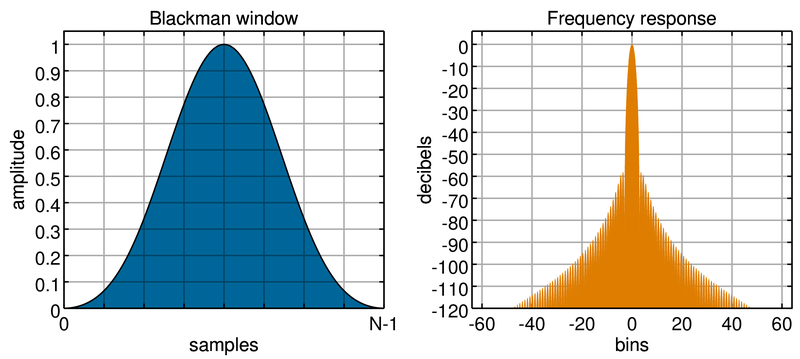
In fact if you just look at the Blackman window : (from Wikipedia)

The window function itself is like a cubic filter. In fact :


Odd Blackman window with half-width of 3 :

const float c_filter[7] = { 0.00660, 0.08050, 0.24284, 0.34014, 0.24284, 0.08050, 0.00660 };

Odd Nutall 3 :

const float c_filter[7] = { 0.00151, 0.05028, 0.24743, 0.40155, 0.24743, 0.05028, 0.00151 };

can be used for filtering by themselves and they're not bad. If you actually want it to work as a *window* , which is just supposed to make your range finite without severely changing your action, it needs to be much wider.

But we don't want to be wide for many reasons. One is the artifacts mentioned previously, the other is efficiency. So, I conclude that you basically don't want all these famous windows.

What you really want for our purposes is something that's flatter in the middle and only get steep at the very edges.


Some windows on 8 taps :

from sharpest to flattest :

//window_nutall :
const float c_filter[8] = { 0.00093, 0.02772, 0.15061, 0.32074, 0.32074, 0.15061, 0.02772, 0.00093 };

//blackman :
const float c_filter[8] = { 0.00435, 0.05122, 0.16511, 0.27932, 0.27932, 0.16511, 0.05122, 0.00435 };

//cos : (aka Hann)
const float c_filter[8] = { 0.00952, 0.07716, 0.17284, 0.24048, 0.24048, 0.17284, 0.07716, 0.00952 };

//window_blackman_sqrt :
const float c_filter[8] = { 0.02689, 0.09221, 0.16556, 0.21534, 0.21534, 0.16556, 0.09221, 0.02689 };

//window_sinc :
const float c_filter[8] = { 0.02939, 0.09933, 0.16555, 0.20572, 0.20572, 0.16555, 0.09933, 0.02939 };

//sin :
const float c_filter[8] = { 0.03806, 0.10839, 0.16221, 0.19134, 0.19134, 0.16221, 0.10839, 0.03806 };

I found the sqrt of the blackman window is pretty close to a sinc window. But really if you use any of these on a filter which is 8-wide, they are severely distorting it.

You can get flatter windows in various ways; by distorting the above for example (stretching out their middle part). Or you could use a parameterized window like Kaiser :


Kaiser : larger alpha = sharper

// alpha = infinite is a delta function
//window_kaiser_6 :
const float c_filter[8] = { 0.01678, 0.07635, 0.16770, 0.23917, 0.23917, 0.16770, 0.07635, 0.01678 };
//window_kaiser_5 :
const float c_filter[8] = { 0.02603, 0.08738, 0.16553, 0.22106, 0.22106, 0.16553, 0.08738, 0.02603 };
//window_kaiser_4 :
const float c_filter[8] = { 0.03985, 0.09850, 0.16072, 0.20093, 0.20093, 0.16072, 0.09850, 0.03985 };
//window_kaiser_3 :
const float c_filter[8] = { 0.05972, 0.10889, 0.15276, 0.17863, 0.17863, 0.15276, 0.10889, 0.05972 };
// alpha = 0 is flat line

Kaiser-Bessel-Derived :

//kbd 6 :
const float c_filter[8] = { 0.01763, 0.10200, 0.17692, 0.20345, 0.20345, 0.17692, 0.10200, 0.01763 };
//kbd 5 :
const float c_filter[8] = { 0.02601, 0.10421, 0.17112, 0.19866, 0.19866, 0.17112, 0.10421, 0.02601 };
//kbd 4 :
const float c_filter[8] = { 0.03724, 0.10637, 0.16427, 0.19213, 0.19213, 0.16427, 0.10637, 0.03724 };
//kbd 3 :
const float c_filter[8] = { 0.05099, 0.10874, 0.15658, 0.18369, 0.18369, 0.15658, 0.10874, 0.05099 };

these are interesting, but they're too expensive to evaluate at arbitrary float positions; you can only use them to fill out small discrete filters. So that's mildly annoying.

There's something else about windowing that I should clear up as well : Where do you put the ends of the window?

Say I have a discrete filter of 8 taps. Obviously I don't put the ends of the window right on my last taps, because the ends of the window are zeros, so they would just make my last taps zero, and I may as well use a 6-tap filter in that case.

So I want to put the end points somewhere past the ends of my discrete filter range. In all the above examples in this post, I have put the end points 0.5 taps past each end of the discrete range. That means the window goes to zero half way between the last tap inside the window and the first tap outside the window. That's on the left :

On the right is another option, which is the window could go to zero 1.0 taps past the end of the discrete range - that is, it goes to zero exactly on the next taps. In both cases this produces a finite window of the desired size, but it's slightly different.

For a four tap filter, the left-side way uses a window that is 4.0 wide ; the right side uses a window that is 5.0 wide. If you image the pixels as squares, the left-side way only overlaps the 4 pixels cenetered on the filter taps; the right side way actually partially overlaps the next pixels on each side, but doesn't quite reach their centers, thus has zero value when sampled at their center.

I don't know of any reason to strongly prefer one or the other. I'm using the 0.5 window extension in my code.

Let me show some concrete examples, then we'll talk about them briefly :


//filter-windower-halfwidth :

//gauss-unity-5 :
const float c_filter[11] = { 0.00103, 0.00760, 0.03600, 0.10936, 0.21301, 0.26601, 0.21301, 0.10936, 0.03600, 0.00760, 0.00103 };

//gauss-sinc-5 :
const float c_filter[11] = { 0.00011, 0.00282, 0.02336, 0.09782, 0.22648, 0.29882, 0.22648, 0.09782, 0.02336, 0.00282, 0.00011 };


//gauss-blackman-5 :
const float c_filter[11] = { 0.00001, 0.00079, 0.01248, 0.08015, 0.23713, 0.33889, 0.23713, 0.08015, 0.01248, 0.00079, 0.00001 };

//gauss-blackman-7 :
const float c_filter[15] = { 0.00000, 0.00000, 0.00015, 0.00254, 0.02117, 0.09413, 0.22858, 0.30685, 0.22858, 0.09413, 0.02117, 0.00254, 0.00015, 0.00000, 0.00000 };

//gauss-blackman-7 , ends cut :
const float c_filter[11] = { 0.00015, 0.00254, 0.02117, 0.09413, 0.22858, 0.30685, 0.22858, 0.09413, 0.02117, 0.00254, 0.00015 };

//gauss-blackman-13, ends cut :
const float c_filter[11] = { 0.00061, 0.00555, 0.03085, 0.10493, 0.21854, 0.27906, 0.21854, 0.10493, 0.03085, 0.00555, 0.00061 };

1. The gaussian, even though technically infinite, goes to zero so fast that you really don't need to window it *at all*. All the windows distort the shape quite a bit. (technically this is a rectangular window, but the hard cut-off at the edge is invisible)

2. Windows distorting the shape is not necessarily a bad thing! Gauss windowed by Sinc (for example) is actually a very nice filter, somewhat sharper than the true gaussian. Obviously you can get the same thing by playing with the sdev of the gaussian, but if you don't have a parameterized filter you can use the window as a way to adjust the compactness of the filter.

3. Cutting off the ends of a filter is not the same as using a smaller window! For example if you made gauss-blackman-7 you might say "hey the ends are really close to zero, it's dumb to run a filter over an image with zero taps at the end, I'll just use a width of 5!". But gauss-blackman-5 is very different! Making the window range smaller changes the shape.

4. If you want the original filter shape to not be damaged too much, you have to use wider windows for sharper window functions. Even blackman at a half-width of 13 (full width of 27) is distorting the gaussian a lot.

4/01/2011

04-01-11 - Dirty Coder Tricks

A friend reminded me recently that one of the dirtiest tricks you can pull as a coder is simply to code something up and get it working.

Say you're in a meeting talking about the tech for your game, and you propose doing a new realtime radiosity lighting engine (for example). Someone else says "too risky, it will take too much time, etc. let's go with a technique we know".

So you go home and in your night hours you code up a prototype. The next day you find a boss and go "look at this!". You show off some sexy realtime radiosity demo and propose now it should be used since "it's already done".

Dirty, dirty coder. The problem is that it's very hard for the other person to win the argument that it's too hard to code once you have a prototype working. But in reality a sophisticated software engineer should know that a demo prototype proves nothing about whether the code is a sensible thing to put into a big software product like a game. It's maybe 1% of the total time you will spend on that feature, and it doesn't even prove that it works, because it can easily work in the isolation of a demo but not be feasible in real usage.

I used to pull this trick all the time, and usually got away with it. I would be in a meeting with my lead and the CTO, the lead would not want some crazy feature I was pushing, and then I would spring it on him that it was "already working" and I'd show a demo to the CTO and there you go, the feature is in, and the lead is quietly smoldering with futile anger. (the most dickish possible coder move (and my favorite in my youth) is to spring the "it's already done, let me show you" as a surprise in the green light meeting).

But I also realize now that my leads had a pretty good counter-play to my dirty trick. They would make me put the risky feature they didn't like in an optional DLL or something like that so it wasn't a crucial part of the normal production pipeline, that way my foolishness didn't impact lots of other people, and the magnified workload mainly fell only on me. Furthermore, optional bits tend to decay and fall off like frostbitten toes every time you have to change compiler or platform for directx version. In that way, the core codebase would clean itself of the unnecessary complicated features.

old rants